Error calculation

Measurement and Uncertainty

Measurement is always accompanied by uncertainty. We distinguish between two main types:

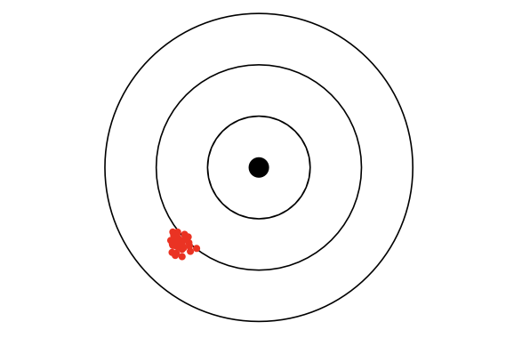
• Systematic uncertainties:

  Systematic uncertainties do influence under the same measurement conditions all measurements in a similar way. Systematic uncertainties are not reducible by repeated measurements.

  

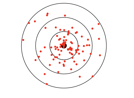
• Statistical uncertainties

  Statistical uncertainties do manifest themselves through random fluctuations around an average value. Statistical uncertainties are reducible by repeated measurements.

  

Empirical mean

The empirical mean of $n$ values $z_i$ of a sample is:

$$ \bar{z} =\frac{1}{n} \sum_{i} z_{i} $$

The empirical mean is best estimate for true value $\left< z \right>$ which remains unknown.

Empirical standard deviation

The empirical standard deviation is the best estimate for true standard deviation $\sigma_z$. It is a measurement of the dispersion of individual measurements around the mean : the smaller the value of $\sigma_z$ , the closer the measurements are to the mean measurement of sample quality

$$ s_{z}=\sqrt{\frac{\sum_{i}^{} \left( \bar{z} -z_{i} \right)^{2}}{n-1}} \simeq \sigma_z $$

Standard error of the mean

$$ s_{\bar{z}} \approx \frac{s_z}{\sqrt{n}} $$

Gaussian probability density

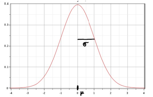
Gaussian probability density with expectation $\mu$ and standard deviation $\sigma$:

$$ f\left( z \right) =\frac{1}{\sqrt{2\pi} \sigma} e^{-\frac{\left( z-\mu \right)^{2}}{2\sigma^{2}}} $$

The expectation $\mu$ corresponds to the true value, the mean $\left< z \right >$.

Graph

The gaussian probability density has the following curve:

Central limit theorem

The central limit theorem states that if a large number of independent and identically distributed random variables are summed, their normalized sum tends toward a Gaussian distribution, regardless of the original distribution of the variables.

Interpretation of standard deviation

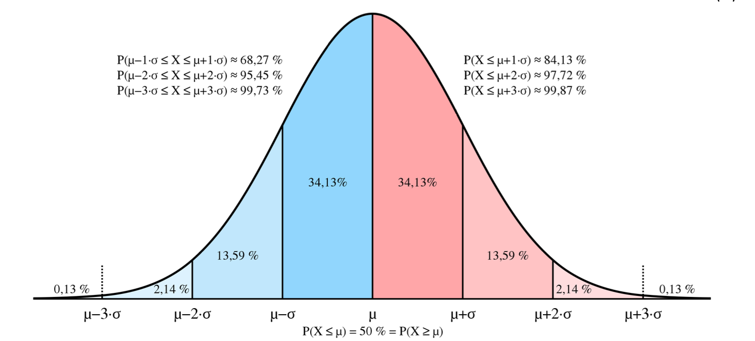
Standard deviation:

• 68,3% of individual values are in the interval $\left< z \right > \pm \sigma_z $

• 95,5% of individual values are in the interval $\left< z \right > \pm 2 \sigma_z $

• 99,7% of individual values are in the interval $\left< z \right > \pm 3 \sigma_z $

Standard error:

• With a probability 68,3% the true value is in the interval $\left< z \right > \pm \sigma_{\left< z \right >} $

• With a probability 95,5% the true value is in the interval $\left< z \right > \pm 2 \sigma_{\left< z \right >} $

• With a probability 99,7% the true value is in the interval $\left< z \right > \pm 3 \sigma_{\left< z \right >} $

Error propagation

Let $R= R(a, b, \cdots)$ be a physical quantity that cannot be measured directly, but which can be calculated from quantities $a, b, \cdots $ measured directly.

Gaussian error propagation law

Definition

For a function $f ( x_1 , x_2 , \cdots , x_n )$ where each variable $x_i$ has an associated uncertainty $\sigma_{x_i}$, the standard deviation or uncertainty of $f$, denoted as $\sigma_f$, can be approximated using a first-order Taylor expansion. The Gaussian error propagation formula is given by:

$$ \sigma_f = \sqrt{ \left( \frac{\partial f}{\partial x_1} \right)^2 \sigma_{x_1}^2 + \left( \frac{\partial f}{\partial x_2} \right)^2 \sigma_{x_2}^2 + \cdots + \left( \frac{\partial f}{\partial x_n} \right)^2 \sigma_{x_n}^2 } $$

Unweighted linear regression

In order to fir a line $y = a + b x$ to minimize the sum of squared deviations between observed and predicted values we use:

\[ \sum (y_i - (a + b x_i))^2 \]

Remark

This method is known as least squares regression. It assumes all uncertainties are equal or negligible.

Weighted linear regression

When measurement uncertainties vary between data points, a weighted least squares approach is used:

\[ \sum \left( \frac{y_i - (a + b x_i)}{\Delta y_i} \right)^2 \]

The weights $1/\Delta y_i^2$ ensure that points with smaller uncertainties contribute more to the fit.

Coefficient of determination $R^2$

The coefficient of determination, often denoted as $R^2$, is a statistical measure that represents the proportion of the variance for a dependent variable that is explained by one or more independent variables in a regression model. It provides an indication of the goodness-of-fit of the model.

Formula

$$ R^2 = 1 - \frac{\sum (y_i - \hat{y}_i)^2}{\sum (y_i - \bar{y})^2} $$

where $ y_i $ are the observed values, $ \hat{y}_i $ are the predicted values from the model, and $ \bar{y} $ is the mean of the observed data.

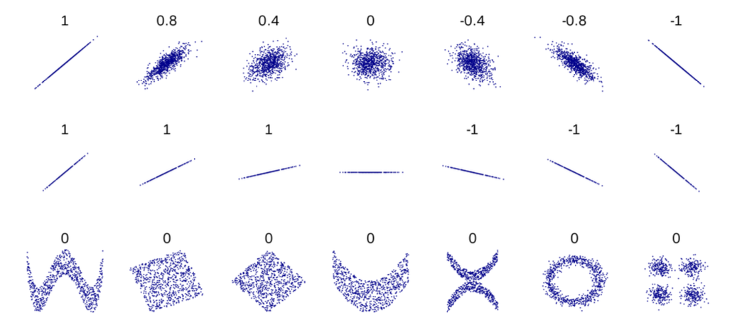
Strength and direction of the coefficient of determination

The correlation coefficient quantifies both the strength and direction, which can be positive or negative, of a linear relationship between an independent variable and a dependent variable.

Range of the coefficient of determination

Range $r$ ranges from -1 to 1:

• An $r$ value of -1 indicates a perfect negative linear relationship: as one variable increases, the other decreases proportionally.

• An $r$ value of 0 suggests no linear relationship between the variables.

• An $r$ value of 1 indicates a perfect positive linear relationship: as one variable increases, the other increases proportionally.

Minimum chi-square estimation

The minimum chi-square estimation involves finding parameter values that minimize the chi-square statistic, which measures the discrepancy between observed and expected data under the model.

Formulas

\[ \chi^2 = \sum \left( \frac{y_i - y_{\text{theory}, i}}{\Delta y_i} \right)^2 \]

The reduced chi-square is:

\[ \chi^2/\text{d.o.f.} = \frac{\chi^2}{\text{degrees of freedom}} \]

A value near 1 suggests that the model describes the data within measurement uncertainties.